Transmission line losses

When designers think of the impedance of a transmission line it has long been commonplace to ignore the losses – and so to a first approximation the impedance of a lossless line can be expressed as:

This is true enough in many cases where the copper is thick enough and the PCB trace wide enough for the losses to be ignored. From an instantaneous point of view the L and C scale per unit length and the ratio of L/C is to all intents and purposes independent of length.

However when geometries shrink, characteristics that could be comfortably overlooked in larger dimensions can no longer be ignored and in that case the equation for transmission lines approximates to:

R is the resistance per unit length, a combination of the DC and AC resistance, and the G is the conductance per unit length. Unlike the L and C, unfortunately, the R and G cannot be seen as dimensionless and the R "piles up" along the trace whilst the G stays close to 0 and the two do not divide out. This means that the TDR impedance trace shows the effect of trace resistance presenting an upward slope as ohm upon ohm of combined DC and AC resistance “pile up” on top of the instantaneous impedance.

Measured v modelled impedance

Without this knowledge someone trying to analyse why the measured impedance is somewhat higher than the prediction may go seeking the source of error. The dimensions are hard to argue with if there is access to precision microsections, especially if three or four sections are taken along the trace and all correlate. So it may be deduced that, given the dimensions are known and provided the impedance measurement system is calibrated and air line verified, that the only unknown is the dielectric constant.

However, deducing that an erroneous Er value is the cause of poor measuring and modeling correlation could be challenged if new facts come to light. Sometimes, the amount Er has to be “adjusted” to make the impedance correlate appears to defy the laws of physics: for example, when the Er is adjusted to a lower level than each of the primary individual constituents of the base material. This should be a clue that something else is awry here.

In 2009 at DesignCon, Navarro, Chairet and Mayevskiy proposed a technique to measure the instantaneous characteristic impedance of high frequency cables by removing the resistive elements through a technique called launch point extrapolation (LPE). The IPC are now looking at applying this to PCB traces for all the reasons described above.

Launch point extrapolation

The benefits of applying LPE to PCB trace impedance test are clear. Linear extrapolation applied to an undisturbed section of the trace and projected back in time to a point close to or at the transition between the probe and the start of the test trace or coupon should remove most of the resistive effects and allow a closer correlation between the modelled impedance and the measured instantaneous impedance. As a precaution and to ensure the copper is not too thin or the line over etched, sometimes, a second point is also measured at an imaginary point at the far end of the trace. This ensures that other effects such as trace taper or a higher than expected copper resistivity are ruled out.

It might be considered that “loss” is catered for when measuring insertion loss in the frequency domain – and this is true – but the types of scenario discussed in this note are those where the lines are operating at “mid” frequencies, i.e. up to one, two or three GHz where the dielectric losses are still small enough to ignore.

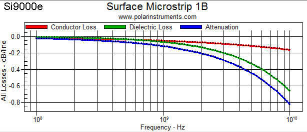
Fig 1  Onset of dielectric loss.

The resistive losses in copper are appearing at these frequencies as a result of the use of thinner copper and narrow line widths. This means that there are small but significant losses from DC upwards. To add to that, the onset of skin effect in copper starts to take effect at lower frequencies than need to be considered in the case of dielectric losses.

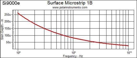
Fig 2  Skin depth

So it is in this “middle ground” of thin copper / narrow traces and low GHz operating speeds that fabricators and designers start to see impedance traces which rise over time (i.e. distance) with the cumulative build up of resistive effects. This effectively means you need to look at the operating frequency band and the trace geometry and the combination of these to choose the most appropriate method for measurement.

So at low frequencies using wide traces – trace capacitance is the predominant issue.

For medium frequencies (1 or 2Ghz) using wide traces – the lossless impedance can be expressed as:

For medium frequencies (1 or 2Ghz) using narrow traces – impedance includes resistance:

For high frequencies (3 GHz and above) – the insertion loss is significant:

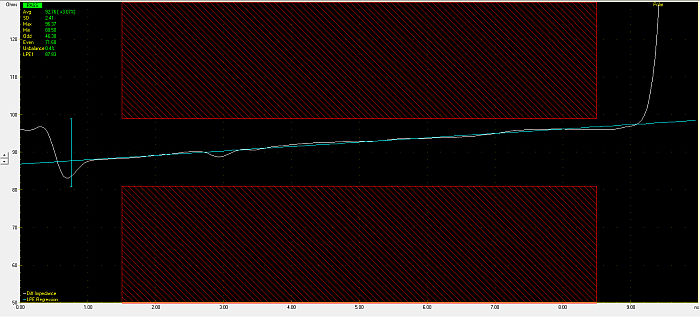
The impedance curve below clearly shows the effect of a long thin narrow copper trace. The slope of the trace over the test region is extrapolated through the LPE point (shown as an error bar near the trace launch point.)

Fig 3  TDR trace with LPE and sloping impedance result.

In conclusion – when looking at transmission line measurements and specifying transmission line characteristics you should ensure that if you are working with narrow traces and thin copper and your frequencies are not yet high enough to need to concern yourself with dielectric losses, you should take a look at your TDR waveforms and if you see a significant slope in the measurement area – consider specifying the measurement of instantaneous impedance by using Launch Point Extrapolation.